PhD: Individually tailored digital-motor outcomes in real life
My Background
My background in Tübingen
Until 2018
B.Sc. in Computer Science
Until 2021
M.Sc. in Computer Science
Until 2024
Research Assistant in Cognitive Science
CCVEP decoding
Tools I like to work with
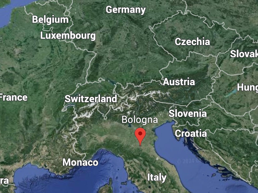
My background in Bologna
Since June 2024
PhD in Health & Technologies
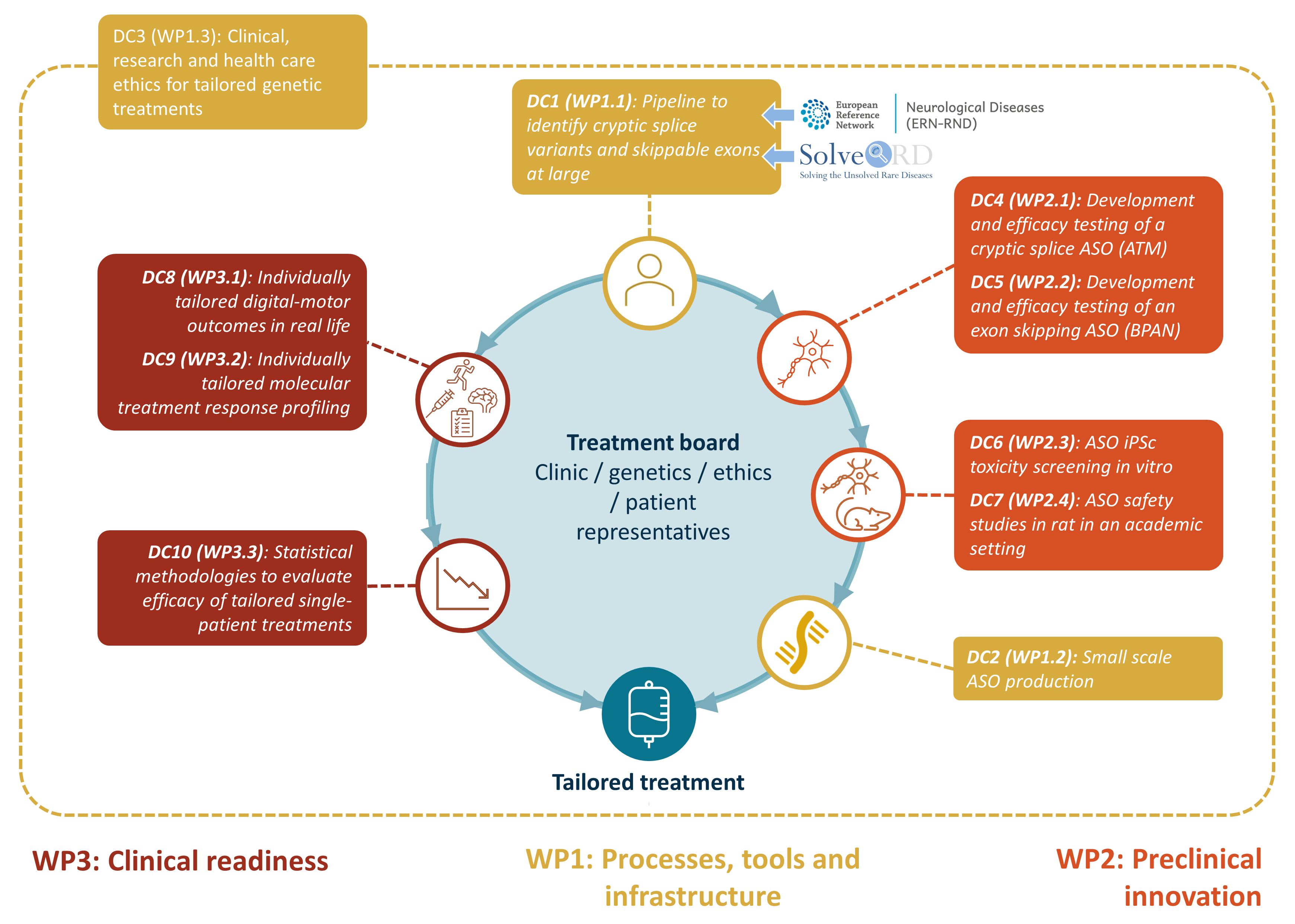
Medicine Made to Measure (MMM)
Doctoral network
Funded by the Marie Curie Actions Scheme
10 PhD candidates
22 participating organisations
Aim: to develop
Antisense oligonucleotide treatments (ASOs)
Tailored to single patients with nano-rare disease mutations
MMM group photos
First General Assembly – Barcelona, June 2024
Mid-Term Meeting – Tübingen, December 2024
Rare diseases
A rare disease is any disease with a
prevalence of <0.05% .
There are >6000 rare diseases.
Taken together, their prevalence is ~4% .
>70% have genetic causes.
Nano-rare mutations: Worldwide
<30 patients.
(approximate numbers, for Europe)
“rare individually, common collectively”
MMM pipeline
Supervisors
Dr. Sabato Mellone University of Bologna
Prof. Dr. Matthis Synofzik University of Tübingen
Prof. Dr. Mats Karlsson University of Uppsala
Co-supervisors
Carlo Tacconi mHealth Technologies s.r.l., Bologna
Prof. Dr. Lorenzo Chiari University of Bologna
Secondments
Tübingen, Germany
Sep 2024 - Nov 2024
Three more months in the coming years
Introduction
Individualized ASOs for nano-rare mutations:
ASO treatment is taylor-made for the mutation
Tiny number of patients worldwide
ASO treatment has slow, disease-modifying effect
Traditional clinical trial designs infeasible
Traditional N-of-1 trial designs infeasible
Spinocerebellar Ataxia (SCA)
Inherited neurodegenerative disease
Affects the cerebellum and spinal cord
Rare disease: ≤5 people per 100,000
Increased gait variability
PhD Objective
Robust assessment of motor performance in genetic ataxias
Based on body-worn sensor recordings in real-life settings
Sensitive to moderate-term change in a single patient
Deliverables
D3.1
Outcomes of the large cohort study Completed Jan 2025
D3.2
Outcomes of focused study Due May 2027 (postponed)
D3.3
Robust capture of n-of-1 movement changes Due Sep 2027
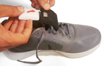
Gait feature extraction
Inertial measurement units
Can be attached to various body parts
Measure movement
Accelerometer
Gyroscope
(Magnetometer, Barometer, …)
Sensor configurations
Lower back and feet
Lower back only
Gait cycle analysis
Gait measures
Gait cycle analysis
Double support
Spatial and temporal analysis
Elevation at mid-swing
Foot contact angles
Circumduction
Lateral step variability
Gait cycle analysis
Spatial and temporal analysis
Elevation at mid-swing
Foot contact angles
Circumduction
Lateral step variability
Walking bouts
Continuous sequences of steps
Delimited by periods of non-walking
Precise definitions vary. Typical criteria:
Minimum length (number of steps, duration)
Maximum allowed pause
Rules for turns
Sanity checks (e.g. consistent left/right alternation)
Walking segments
Split long walking bouts evenly into segments ≥25 strides.
Better temporal resolution and homogeneity
Additional features
Signal
Position
Left foot
Right foot
Trunk
×
×
Quantity
Acceleration
Angular velocity
(Magnetometer)
(Barometer)
×
↓
↓
Feature classes
Stride-to-stride comparisons
Discrete transform coefficients
Cumulative (absolute) signal
…
↓
Window
Walking bout
Walking segment
↓
Feature classes
Complexity measures
Cumulative (absolute) signal
…
Stride-to-stride comparisons
Discrete transform coefficients
Complexity measures
Feature aggregation
Aggregate:
Lateral feature pairs (left foot and right foot)
Stride-wise features in each walking segment
Segment-wise features in each session/condition
Possible aggregators:
Arithmetic mean
Standard deviation
Coefficient of variation
Median, quantiles, extrema
Interquantile ranges
Quartile coefficient of dispersion
…
Result: Many candidate outcomes, each with one value per
subject and session/condition
Feature transformation
Transform features on the per-stride, per-segment, or
per-session/condition level.
Possible transformations:
Absolute value
Normalization (e.g. by body height)
n th-order differences
Logarithm
…
Why transform? Examples:
We are interested in an absolute deviation, not its direction
We are interested in stride length relative to body height
We are interested in the difference between two strides
We want to compare multiplicative factors
…
Environmental context effects
Real-life context factors are known to affect gait features
Indoors vs. outdoors
Type or absence of shoes
Slope, stairs
Ground texture
Weather
…
Exogenous variables, introducing variance
Estimateable to some degree from signal-derived proxies
Context stratification
Approach:
Stratifiy walking segments by context proxies
Obtain one candidate outcome per stratum
Stratum intersections or unions possible too
Keywords
Covariate
Threshold(s)
slow /
fast
Gait speed
1.2m/s
sporadic /
continuous
Number of steps in a 1-minute window
45
straight /
curvy
Number of turns in a 1-minute window
1
short /
long
Walking bout duration
30s
Disadvantages:
High feature count gets increased even more
The more specific a stratum, the less data is considered
Context compensation
Approach:
Fit a linear model for each per-segment feature
Dependent variable: Feature
Regressors: Context proxies
Explain context-induced variance
Without touching disease-status-induced variance
Gait feature extraction summary figure
Data
Dataset
Gait recordings from Tübingen University Hospital
27 genetic spinocerebellar (pre-)ataxia patients
36 healthy controls
Lab-based & real-life
Yearly follow-ups over several years
Patients further categorized into:
6 pre-symptomatic (SARA 2 ± 1)
21 symptomatic (SARA 10 ± 3)
In total:
~200 visits
~20000 walking segments
~570,000 gait cycles
Other potential datasets
PROSPAX
Lab-based movement recordings only
≥74 ARSACS (spastic ataxi) patients
≥113 SPG7 (spastic paraplegia) patients
≥50 healthy controls
Planned prospective study
≥10 ataxia (SCA or AT) patients
Outcomes
Clinician- / patient-rated scores (per visit)
SARA
ABC
Others, but incomplete (SPRS, INAS, PGI, ADL)
Digital motor outcomes
Large space of combinations, small fraction suitable
Further covariates
Demographics (age, gender)
Diagnosis / gene affected
Anthropometrics at first visit (weight, height, handedness, …)
Estimated age of disease onset (only 19 of 27 patients)
SARA score
“Scale for the assessment and rating of ataxia”
Item
Possible responses
1) Gait
0 - 8
2) Stance
0 - 6
3) Sitting
0 - 4
4) Speech disturbance
0 - 6
5) Finger chase
0 - 4
6) Nose-finger test
0 - 4
7) Fast alternating hand movements
0 - 4
8) Heel-shin slide
0 - 4
Total
0 - 40
ABC score
“Activities-specific balance confidence scale”
How confident are you that you will not lose your balance or become
unsteady when you…
…walk around the house?
…walk up or down stairs?
…bend over and pick up a slipper from the floor?
…
Traditionally 16 items
In the Tübingen dataset: extended to 41 items
Disease onset estimates
Tezenas du Montcel et al. 2014
Data: Per-visit level
SARA scores in healthy subjects simulated (based on Shaafi Kabiri et al.
2018)
Data: Per-visit level
SARA scores in healthy subjects simulated (based on Shaafi Kabiri et al.
2018)
Qualitative characteristics
Generally constant over time in the absence of disease
Effect of age, if present, is small
Roughly linear rise at disease onset
Theoretical saturation not/barely represented in the dataset
Clinical scales bounds not reached
DMOs said to saturate around SARA 12-15
Data are potentially “ill-behaved” in several ways:
Selection/attrition bias
Disease onset estimation error (and missingness)
Depending on model, residuals might be:
Heteroskedastic
Non-normal
Serially correlated
Data: Per-segment level
Cross-sectional testing
Paired-samples testing
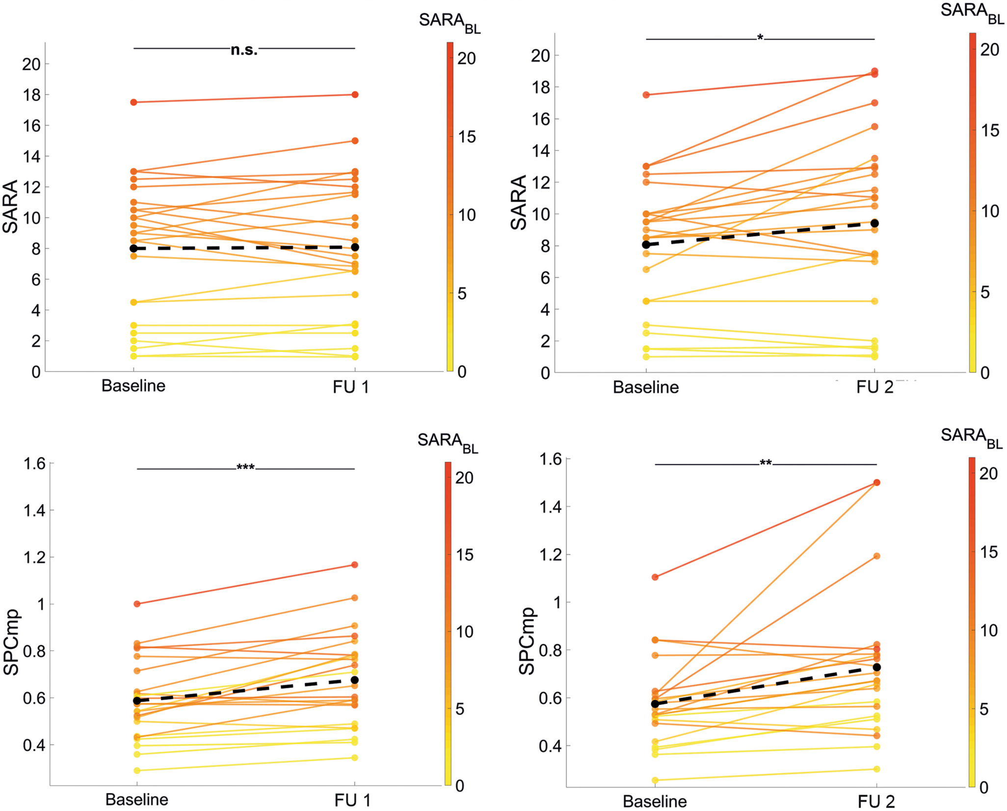
Longitudinal paired-samples testing (Seemann
et al.)
Seemann et al. 2025
Longitudinal paired-samples testing (Seemann
et al.)
Seemann et al. 2025
Longitudinal paired-samples testing
Longitudinal paired-samples testing
Longitudinal paired-samples testing
Longitudinal paired-samples testing
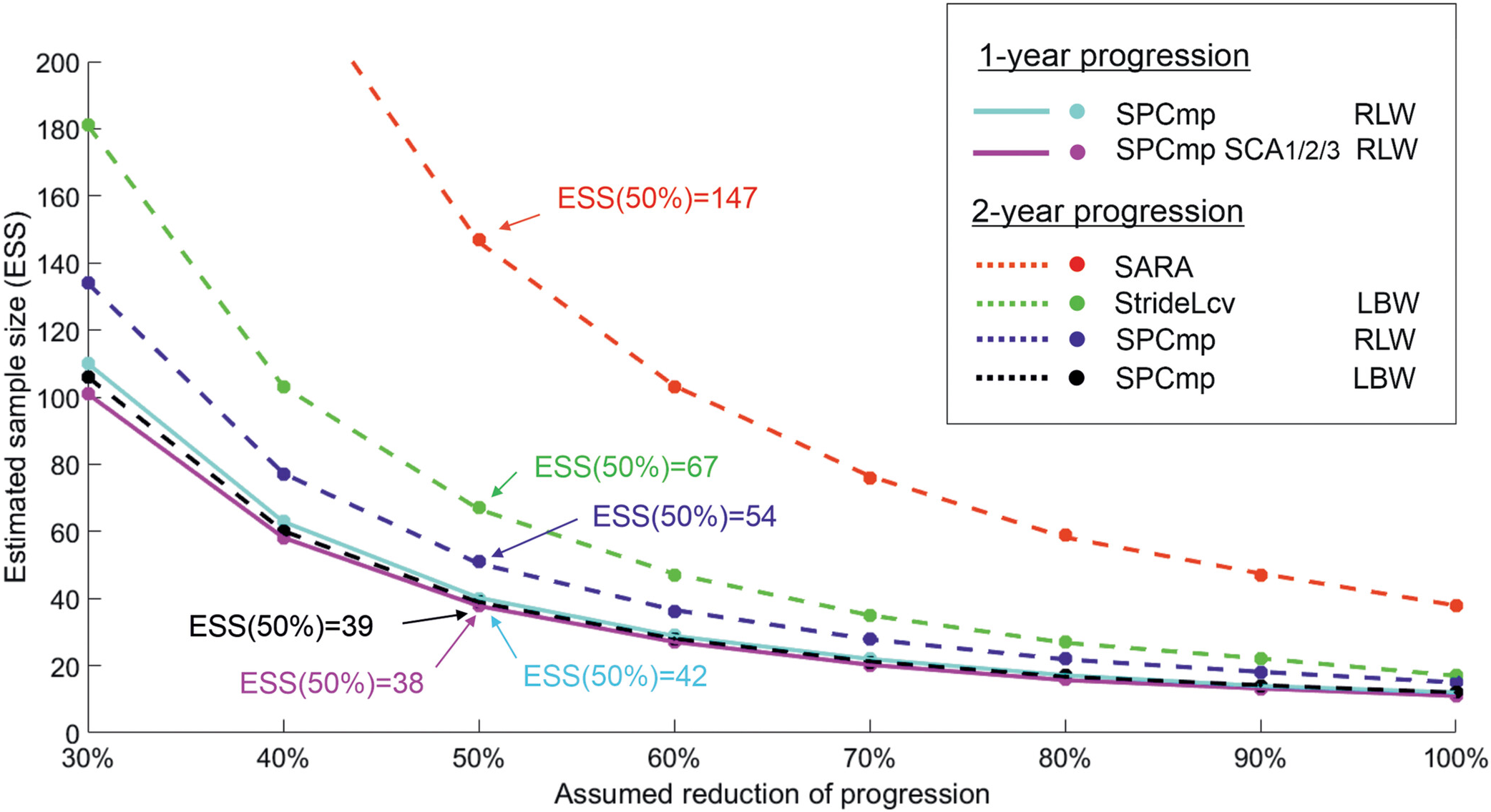
Pooled sample size estimates
TODO: Focused disease range, new pooling
Pool 1-, 2-, and 3-year effect sizes
With inverse variance weighting
Pre-normalize to 1-year by linear interpolation
Assumes outcomes change linearly on average
Panel model of outcome trajectories
Panel model
\[
y_{ij} = \beta_1\mathrm{BOn}_{ij} + \beta_2\mathrm{BSat}_{ij} +
\beta_3\mathrm{BOn}_{ij}\left(\mathrm{EDO}_\mathrm{o}\right)_{i} +
\beta_4\mathrm{BOn}_{ij}\mathrm{Gender}_{i} +
\beta_4\mathrm{BOn}_{ij}\mathrm{BMI}_{i}
\]
Fixed-effects panel model (= linear model with de-meaning)
Done as a course exercise
Non-parametric bootstrap & Monte Carlo methods employed
Fixed-effects panel model predictions
Fit results
Outcome (lab-based)
gait_speed_apdm_μ/μ/all/μ
stride_length_apdm_μ/cv/all/μ
\(R^2\)
0.60
0.50
\(\mathrm{BOn}\) (\(p\))
-0.011 (0.92)
0.0083 (0.32)
\(\mathrm{BSat}\) (\(p\))
-0.22 (2.2e-07)
0.012 (0.00035)
\(\mathrm{BOn} \times \mathrm{Gender}\) (\(p\))
-0.095 (0.00028)
0.0044 (0.041)
\(\mathrm{BOn} \times \mathrm{BMI}\) (\(p\))
-0.0061 (0.10)
6e-04 (0.054)
\(\mathrm{BOn} \times \mathrm{EDO_o}\) (\(p\))
0.0043 (0.00013)
-0.00053 (5.3e-08)
ESS
60
106
ESS (Seemann et al. 2025)
66
67
Simulating outcome data
Data-generating process:
Fix the number of patients and controls.
Draw uniform ground-truth time since disease onset for first
visit.
Scale time since disease onset by log-normal variation to model
ground-truth severity.
Simulate selection bias by discarding patients above a fixed
severity threshold.
Simulate normal disease onset estimate error in approximate
accordance with Tezenas du Montcel et al. 2014.
Draw uniform number of visits per subject.
Create time intervals with normal error and extrapolate
time-varying variables.
Transform ground-truth severity by basis functions imitating
soft onset and feature saturation behavior.
Add non-normal, serially correlated residuals with differing pre-
and post-onset variance.
Simulating outcome data
Assumption violations
Here:
Simulated data
No bootstrapping
Random-slope modeling
Model overview
Subject-centered growth model
The “minimal” longitudinal mixed-effects model
\[
y_{ij} = \beta_0 + \beta_1 \tilde{x}_{ij} + b_{0i} +
b_{1i} \tilde{x}_{ij} + \epsilon_{ij}
\]
\[
\begin{pmatrix}
b_{0i} \\
b_{1i}
\end{pmatrix}
\sim
\mathcal{N}\!\left(
\begin{pmatrix}
0 \\
0
\end{pmatrix},
\begin{pmatrix}
\sigma_{b0}^2 & 0 \\
0 & \sigma_{b1}^2
\end{pmatrix}
\right),
\qquad
\varepsilon_{ij} \sim \mathcal{N}(0, \sigma^2)
\]
Where:
\(i\) enumerates subjects, \(j\) enumerates visits
\(\tilde{x}_{ij} = x_{ij} - \bar{x}_i\) is subject-centered time
(or clinical scale to compare against)
\(\beta_0\) and \(\beta_1\) are the fixed intercept and slope
\(b_{0i}\) and \(b_{1i}\) are the random intercept and slope for
subject \(i\)
Random-slope model fit
Outcome ranking
Outcome ranking
TODO: Update outcome ranking
outcome
ess
rb_lgt
rb_crs
ρ_ΔΔ_2y
spread
1y
2y
3y
sym
sara<8
sara≥8
sara
-abc
test_dw_instance_compound_5 39
.86 .75 .96 .68 .28 .67 .32 .12
test_dw_instance_compound_3 45
.82 .66 .93 .59 .18 .62 .26 .26
test_dw_instance_compound_2 55
.77 .78 .78 .49 .36 .48 .58 .21
test_dw_instance_compound_4 66
.79 .65 .36 .75 .48 .52 .33 .2
agg_adjacent_swings_resampled_sensor_lumbar_acc_x_r_d1_abs_μ /σ /curvy_long /μ 74
.71 .45 .76 .52 .32 .46 -.5 -.06 .47
agg_adjacent_swings_resampled_sensor_lumbar_acc_x_r_μ /σ /curvy_long /μ 83
.62 .62 .67 .54 .24 .45 -.32 .0055 .45
agg_adjacent_swings_resampled_sensor_lumbar_gyr_z_r_abs_μ /σ /long /μ 86
.68 .46 .54 .5 .066 .42 -.036 .2 .52
agg_adjacent_swings_resampled_sensor_lumbar_gyr_z_r_abs_d1_abs_μ /σ /long /μ 88
.72 .4 .41 .49 .09 .4 .062 .32 .57
agg_adjacent_swings_resampled_sensor_lumbar_acc_x_r_abs_μ /σ /curvy_long /μ 88
.58 .66 .65 .54 .24 .45 -.3 .21 .42
agg_adjacent_swings_resampled_sensor_lumbar_gyr_z_r_abs_d3_abs_μ /σ /long /μ 89
.71 .42 .38 .48 .067 .41 .11 .093 .54
stance_duration_μ /cv /curvy_long /μ 90
.65 .76 .38 .63 .29 .52 .25 -.43 .45
agg_adjacent_swings_resampled_sensor_lumbar_gyr_z_r_abs_d2_abs_μ /σ /long /μ 93
.71 .44 .38 .48 .067 .4 .11 .21 .54
agg_adjacent_swings_resampled_sensor_lumbar_gyr_z_r_abs_d1_abs_μ /μ /long /μ 94
.62 .52 .43 .54 .12 .42 .16 .31 .44
double_support_apdm_μ /σ /curvy_long /μ 95
.69 .46 .49 .72 .42 .46 .13 -.37 .36
coeff_swings_sensor_acc_dft_x_1_abs_μ /cv /long /μ 95
.76 .51 .43 .71 .43 .44 .1 .044 .41
agg_adjacent_swings_resampled_sensor_lumbar_acc_x_r_abs_d2_abs_μ /μ /curvy_long /μ 96
.66 .5 .56 .63 .32 .49 -.24 .088 .42
agg_adjacent_swings_resampled_sensor_lumbar_gyr_z_r_abs_d3_abs_μ /μ /long /μ 97
.65 .49 .43 .54 .12 .42 .24 .35 .46
swing_apdm_μ /cv /curvy_long /μ 98
.72 .58 .49 .7 .36 .51 .15 -.32 .36
agg_adjacent_swings_resampled_sensor_lumbar_gyr_z_r_abs_d2_abs_μ /μ /long /μ 98
.64 .51 .41 .53 .11 .42 .22 .31 .43
agg_adjacent_swings_resampled_sensor_lumbar_acc_z_r_abs_d3_abs_μ /γ /short /μ 98
-.69 -.53 -.41 -.48 -.28 -.48 -.57 -.15 .69
agg_adjacent_swings_resampled_sensor_lumbar_acc_x_r_abs_d1_abs_μ /σ /curvy_long /μ 100
.66 .45 .69 .51 .31 .44 -.49 .071 .42
initial_plus_mid_swing_apdm_μ /cv /curvy_long /μ 100
.63 .69 .6 .67 .42 .42 -.097 .082 .38
agg_adjacent_swings_resampled_sensor_lumbar_gyr_z_r_abs_μ /cv /long /μ 100
.57 .56 .47 .5 .072 .41 .1 .15 .57
gait_speed_apdm_μ /σ /curvy_long /μ 100
.57 .73 .34 .44 .21 .45 .39 0 .42
(…)
sara_sim_1 103
.53 .56 .76 1 .85 1 1 .077
(…)
Outcome ranking: Metrics
TODO: Update metrics
ess
1-year estimated sample size (pooled from 1-, 2-, 3-year)
rb_lgt
Longitudinal effect sizes (Wilcoxon signed-rank rank biserial)
rb_crs
Cross-sectional effect sizes (Mann-Whitney rank biserial)
ρ_ΔΔ_2y
2-year change correlation (Spearman)
spread
Measure of within-visit variation
Outcome ranking: Filtering
TODO: Update filtering
Require:
A certain ability to discriminate symptomatic patients
A certain ability to discriminate low-SARA from higher-SARA
Longitudinal patient p-values to be (somewhat) significant
Reasonable number of patients considered longitudinally
Longitudinal effects in controls to be non-significant or small
Longitudinal and cross-sectional effects' signs to agree
Composite measures
Why composite measures?
Many candidate outcomes, capturing variance from:
Various aspects of disease severity
Various nuisance factors
Combining them into a composite score could:
Leverage orthogonal information from different features
Average out some of the unwanted variance
Similar to a test battery for a clinical score
Optimized composite measures
Idea: Formulate the search for the ideal combination of outcomes
as an optimization problem.
E.g. Find linear combination that minimizes some loss.
Loss: E.g. Composite change vs. disease time change.
\[
\min_\beta \sum_{i, j} \left(
\left( t_{i j} - \bar{t}_{i \cdot} \right) \cdot
I_{\mathrm{symptomatic}}(i) -
\sum_{k} \left( y_{k i j} - \bar{y}_{k i \cdot} \right) \cdot \beta_k
\right)^2 + \Omega(\beta)
\]
This is a linear regression (with optional regularizer
\(\Omega(\beta)\))
From the de-meaned (and normalized) per-visit outcomes
To the de-meaned time since baseline, if symptomatic
Result \(\theta = \beta y\) is a generated regressor – likely
suboptimal compared to a jointly estimated latent variable model.
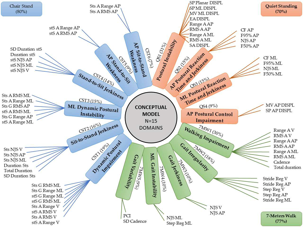
Factor analysis
The “original” latent variable model
Distills a set of observed variables into a few conceptual
factors
Coni et al. 2019
Pilot test on visit level resulted in subpar composites
Cross-sectional latent disease severity modeling
Cross-sectional latent disease severity
modeling
Model disease severity itself
Using a non-linear, single-factor, latent variable model
Cross-sectionally, on the segment level
Use established relationships between features and severity for a
longitudinal model
This has been done with success recently by Hamdan et al.
On lab-based, visit-level features + SARA score
Item characteristic curves (Hamdan et al.)
Hamdan et al. 2024
Fisher information (Hamdan et al.)
Hamdan et al. 2024
ccIRT model performance (Hamdan et al.)
Hamdan et al. 2025
ccIRT model performance (Hamdan et al.)
Hamdan et al. 2025
Model overview
Bayesian non-linear single-factor model
“Cross-sectional”, i.e. considers each visit as an
individual
Relates segment-level features to the latent disease severity
By fitting a non-linear function per feature
No incorporation of clinical scores
\[
y_{ij} = f\left(s_{v(i)}, \gamma_j\right) \, \beta_j + \alpha_j +
\epsilon_{ij} \qquad \epsilon_{ij} \sim t_\nu\left(0,
\sigma^2_j\right), \, s_v \sim \mathcal{N}(0, 1)
\]
Where:
\(j\) enumerates features
\(i\) enumerates walking segments
\(v(i)\) is the visit to which walking segment \(i\) belongs
\(s_{v(i)}\) is the severity at visit \(v(i)\)
Choice of \(f\)
\[ \begin{align}
\mathrm{exprel}(x) &= \frac{e^x - 1}{x} \\
\mathrm{tilt}(x, \gamma) &= x \, \mathrm{exprel}(\gamma x) \\
f(x, \gamma) &= \mathrm{tilt}(x, \gamma) \, \mathrm{scale}(\gamma) +
\mathrm{offset}(\gamma)
\end{align} \]
Where \(\mathrm{scale(\gamma)}\) and \(\mathrm{offset}(\gamma)\) are
deterministic functions of \(\gamma\) chosen such that
\[
x \sim \mathcal{N}(0, 1) \Rightarrow
\mathrm{E}\left[f(x, \gamma)\right] = 0,
\mathrm{Var}\left[f(x, \gamma)\right] = 1
\]
\(\gamma\) becomes a shape parameter that does not affect the
offset and scale of \(x\)
Choice of residual prior
\[
\epsilon_{ij} \sim t_\nu\left(0, \sigma^2_j\right)
\]
Where
\[ \begin{align}
\log \sigma_j &\sim \mathcal{N}\left(\mu_\sigma,
\sigma^2_\sigma\right) \\
\mu_\sigma &\sim \mathcal{N}\left(\log \mu_{\mu_\sigma},
\left(\frac{\log \sigma_{\mu_\sigma}}{1.96}\right)^2\right) \\
\log \sigma_\sigma &\sim \mathcal{N}\left(\log \mu_{\sigma_\sigma},
\left(\frac{\log \sigma_{\sigma_\sigma}}{1.96}\right)^2\right)
\end{align} \]
And e.g.
\[
\mu_{\mu_\sigma} = 0.8 \qquad
\sigma_{\mu_\sigma} = 1.5 \qquad
\mu_{\sigma_\sigma} = 0.3 \qquad
\sigma_{\sigma_\sigma} = 1.6
\]
Hierarchical prior with feature-specific scale
\(t\)-distributed residuals for robustness against outliers
Choice of parameter priors
\[ \begin{align}
\alpha_j &\sim \mathcal{N}(0, \sigma^2_\alpha) \\
\beta_j &= \mathrm{softplus}(\eta_j, \delta) \qquad
\eta_j \sim \mathcal{N}(\mu_\eta, \sigma^2_\eta) \\
\gamma_j &\sim \mathcal{N}(0, \sigma^2_\gamma)
\end{align} \]
Where e.g.
\[
\sigma_\alpha = 0.5 \qquad
\mu_\eta = -1 \qquad
\sigma_\eta = 0.7 \qquad
\sigma_\gamma = 0.5 \qquad
\delta = 1
\]
And
\[
\mathrm{softplus}(x, \delta) = \max(x, 0) + \log\left(1 +
e^{-\frac{|x|}{\delta}}\right) \, \delta
\]